Every MSAT's Response to Process Development

Reducing variability is the only thing the Manufacturing team can control.  Ways to do this involve getting more accurate probes, improving control algorithms, upgrading procedures, etc.

But there are limits. Probes are only so precise. Transmitter may discretize the signal and add error to the measurement. The cell culture may have intrinsic variability.

What makes for releasable lots are cell cultures executed within process specifications.  And measuring a process parameter's variability in relation to the process specification is the SPC metric: capability.



Process specifications are created by Process Development (PD). And at the lab-scale, it's their job to run DOE and explore the process space and select process specifications narrow enough to produce the right product, but wide enough that any facility can manufacture it.

by Oliver Yu

It's tempting to select the ranges that produce the highest culture volumetric productivity.  But that would be a mistake if those specifications were too narrow relative to the process variability.  You may get 100% more productivity, but at large-scale be only able to hit those specifications 50% of the time resulting in a net 0% improvement.

The key is to pick specification limits (USL and LSL) that are wide so that the large-scale process is easy to execute.  And at large-scale, let the MSAT guys find the sweet-spot.

How To Interpret Distributions (Histograms)

Here's a set of Y-Distributions (histograms) I saw on the data visualization sub-Reddit.

On the left side, we have Polish language scores. On the right, we have mathematics.

Each row is a year... 2010 through 2012.

According to the notes on the page, these are the high-school exit exam scores for which passing is to receive 30% of the total available points.


Most people know what a "bell-shaped" curve looks like and those Polish language scores don't look like bells. In fact, it looks like right around the 30% mark, someone took the non-passing scores that were "close enough" and just handed out the passing score.

We sometimes see this in biotech manufacturing... where in order to proceed to the next step, you need to take a sample and measure the result. If there is a specification, you'll see a lot of just-passing results. What is euphemistically called, "Wishful sampling."

The process is the process and if the sampling is random, you expect a bell-shaped curve. In the case of Polish high school students, their Polish skills are what they are. What you're seeing is an artifact of the people grading the tests. I would bet a fair amount of money that teachers or schools are rewarded according to the number of students who pass this test.

Let's look at the mathematics scores. This "wishful grading" is going on in mathematics, but is far less pronounced. What is crazy is how different the distributions look from year to year (compared to the language histograms).

It's hard for me to think that mathematics skills of students across Poland vary that much from year to year. Like the U.S. News and World Reports rankings of schools, it's more likely that the difficulty of the test changes significantly from year to year... in this case with 2011 tests with particularly difficult questions.

by Oliver Yu

Histograms say quite a bit about your process. What they never tell you is that the histograms also tell you quite a bit about your process specifications and how truthful your measurement systems are.

If I were the FDA... and I wanted to be mean about it, I'd request a distribution of measurements for every single process specification, and if I saw something like this "Polish language" test, someone has some explaining to do.


Get Biotech Manufacturing Consulting

Dr. Tom Little - Stats Ninja

by Oliver Yu

There is an epidemic of statistical dunderheads working in the biotech industry. This epidemic probably plagues other sectors of the economy as well, but I'm not qualified to speak to that.

The reason for this complete lack of statistical knowledge (I think) is that statistics is not a part of the standard engineering curriculum. You get differential and integral calculus like crazy, but just one semester of basic engineering statistics and here's your diploma.

And as with most of undergraduate academia, it's not practical.

At my first job, we used the statistical software program - JMP - a lot. We were making a minimally invasive glucose monitor called the, GlucoWatch® Biographer and my entire job as a research engineer was to run in-house clinical studies and correlate the biographer performance against over-the-counter glucose meters. So we did a lot of linear correlations, I got to understand what p-values meant. And I figured out the primary purpose of engineering a system was to figure out what was signal and what was noise.

I think I might have even landed my second job because I knew how to use JMP. In fact, my second week on the job, the boss had his entire group go get JMP training in San Francisco where I had the luck of sharing a computer terminal with him.

Whatever the case, understanding enough statistics to know what tests are applicable when is really important. And when your group gets big enough that sending your team to off-site training becomes impractical, there is Dr. Thomas Little who will send practical stats gurus to train you.




Dr. Tom trained us (in a computer room) setting and a lot of this stuff was new at the time I learned it. ANOVA... Multivariate Analysis. Why use backwards stepwise regression... how to read the normal quantile plot... Capability... Control Charting.... All the things that are relevant to monitoring a production campaign.

When you get out of the class, you've leveled up in the world of biologics manufacturing and you look around and wonder why maintaining spreadsheets of cell culture data qualifies as plant support. You also start wondering why process development spends more time swinging male genitalia over higher titers rather than defining critical process parameters (CPPs) and identifying proven acceptable ranges (PARs).

Dr. Tom is pretty well-known in the world of biologics. I run into his team of consultants every third place I go. If your team isn't making statistically-sound, data-drive decisions, you seriously need to give him a call.

Call Dr. Tom

@zymergi

Manufacturing Sciences: Campaign monitoring v. Process Improvement

by Oliver Yu

Manufacturing Sciences is the name of the department responsible for stable, predictable performance of the large-scale biologics process.

Manufacturing Sciences also describes the activities of supporting for-market, large-scale, GMP campaigns. The three main functions of Manufacturing Sciences are:

1. Campaign monitoring
2. Long-term process improvement
3. Technology Transfer

Within the department are:

1. Data analysis resources - responsible for campaign monitoring
2. Lab resources - responsible for process improvement

Figure 1: Flow of information within Manufacturing Sciences

The data group is responsible for monitoring the campaign and handing off hypothesis to the lab group.  The lab group is responsible for studying the process under controlled conditions and handing off plant trials back to the data group.

Campaign Monitoring

When a cGMP campaign is running, we want eyeballs watching each batch. There are automated systems in place to prevent simple excursions, but on a macro level, we still want human eyeballs. Eyeballs from the plant floor are the best. Eyeballs from the Manufacturing Sciences department are next best because they come with statistical process control (SPC) tools that help identify common and special cause.

Activities here involve:

• Defining key performance indicators (KPIs) for inoculum and production cultures.
• Control charting these KPIs
• Computing process capability.
• Running univariate and bivariate analysis

Ultimately, all this statistical process control enables data-based, defensible decisions for the plant floor and to production management, much of which will involve the right decisions for decreasing process variability, increasing process capability and reliability.

Long-term Process Improvement

The holy-grail of manufacturing is reliability/predictability. Every time we turn the crank, we know what we're going to get: a product that meets the exact specifications that can be produced with a known quantity of inputs within a known or expected duration.

Long-term process improvement can involve figuring out how to more product with the same inputs. Or figuring out how to reduce cycle time. Or figuring out how to make the process more reliable (which means to reduce waste or variability.

This is where we transition from statistical process control to actual statistics. We graduate from uni- and bivariate analysis into multivariate analysis because biologics processes have multiple variables that impact yield and product quality. To understand where there are opportunities for process improvement, we must understand the system rather than simple relationships between the parts. To get this understanding, we need to have a good handle on:

• Multivariate Analysis
• Multiple Linear Regression

Note: in order to have a shot at process improvement, you need variable data from large-scale. Meanwhile if you succeed at statistical process control, you will have eradicated variability from your system.

This is why a manufacturing sciences lab is the cornerstone of large-scale, commercial process improvement - so that you can pursue process improvement without sacrificing process variability and the results of your statistical process control initiatives.

Outsource Manufacturing Sciences

Toyota visits Zymergi(.com)

This is pretty flattering. Someone from Toyota - the creators of Toyota Production System... which is the precursor to Lean... looked up Process Capability (CpK) on Google and read my blog post:


I'm pretty excited. When you study manufacturing and look for the words of truth that apply across industries, Toyota is the leader in quality. Competing with limited resources and applying the principles that Deming taught them, they went from post-World-War 2 clothmaker to the largest automobile company on planet Earth.

How to Make IR Control Charts

by Oliver Yu

Suppose you support a batch process. The way you likely measure performance is to sample each batch and measure different parameters. These measurements are ideal for plotting on an IR control chart - one control chart for each parameter and each batch would be represented by one point on the control chart.

If you have statistical software like JMP, then you can just click around on the menu



...and...



control charts appear like magic:



But suppose Wall Street bankers crashed the economy by securitizing AAA-rated subprime mortgages and you are the collateral damage; forking over $1,250 for a single-user annual license or $1,895 for a single-user perpetual license of JMP isn't in the cards. What do you do?

Good news. William Shewhart developed control charting principles long before computers so if worse comes to worse, you could probably create a control chart from graph paper and a grease pencil.

Here's what you do:

1. Get the data into a column
2. Compute moving range
3. Multiply MR by 3 and divide by 1.128

We're not going to do it with a grease pencil and graph paper. We're going to do it with a spreadsheet.

Step 1: Get the data into a column

We haven't talked about this yet, but data for analysis needs to be structured. If you look at the numbers in a column and they represent what the column headers describe, then you got it right.

Step 2: Compute the Moving Range

This is where you take the absolute value of the difference between measurements. =B3-B2 would be the formula that you'd drag in column C. The average of the moving range is used to determine the width of the control limits.

Step 3: Compute distance to control limits

To get the distance to each control limit, compute 3 * Average( MovingRange ) / 1.128.



In this case, the average of the moving range is 3.90. Take 3.90 * 3 / 1.128 = 10.37.

The Upper Control Limit (UCL) is the 296 + 10.37 = 306

The Lower Control Limit (LCL) is the 296 - 10.37 = 286

What you do is calculate limits for every parameter you measure; apply it to a steady process and lock the limits and monitor the process against the locked-down limits to detect drift.

Get Control Chart Experts

Continuous Process Improvement and SPC

by Oliver Yu

Buzzwords are aplenty in this line of work: Lean manufacturing, lean six sigma, value stream mapping, business process management, Class A. But at the end of the day, we're talking about exactly one thing: continuous process improvement:

How to get your manufacturing processes (as well as your business process) to be better each day.

And to that, I say: "Pick your weapon and let's get to work." For me, I prefer statistical process control because SPC was invented in the days before continuous process improvement collided with information technology.

Back in those days, things had to be done by hand, concepts had to be boiled down in simple terms: special cause vs. common cause variability could simplify what was going on and clarify decision making. And having just Excel spreadsheets is a vast technological improvement to paper and pencil. In those days, there was no time for complexity of words and thought.

If we say words from the slower days of yesteryear, but use tools from today, we can solve a lot of problems and make a lot of good decisions.

Companies like Zymergi are third-party consultants who can help develop your in-house continuous process improvement strategy; especially for cell culture and fermentation companies. We focus applying statistical process control as well as knowledge management so that once we reduce process variability and increase reliability.

The technology is there to institutionalize the tribal knowledge so that when people leave, your high-paid consultants leave, the continuous process improvement know-how stays.

We use SPC and statistical analysis because it has been proven by others and it is proven by us. Data-driven decisions deliver real results.

7 Tools of SPC

1. Control Charts
2. Histograms
3. Correlations
4. Ishikawa Diagrams
5. Run Charts
6. Process Flow Diagrams
7. Pareto Charts

Control Chart Limits vs. 3 StDev

by Oliver Yu

While control limits are approximations of 3 standard deviations, they are not 3 standard deviations.

In thermodynamics, we talk about state variables and path variables. State variables - like internal energy (U) … "is what it is." Other variables like work (w) are path variables… "its value depends on how you got there."

Standard deviation is a "state"-like parameter… if you have a set of points, the standard deviation is the standard deviation; it does not matter the order in which the data happened.



Using the same data from our previous control charting example, we see the standard deviation is 2.9 and a mean of 295. The 3 standard deviations around the average is 286 - 303.

Control limits, on the other hand, are path-like parameters that depend on the order in which it was received, and in the case of pretty random data, the control limits are 285 - 306... which is pretty close to the 3 standard devations, but not exact.




Viewing the control chart, it's obvious there are no special cause signals and there are no patterns in the data that indicate the data is out of the ordinary.

But suppose we got the same exact measurements... except this time, we found that each observed value was equal to or higher than the previous:




The standard deviation remains the same and therefore average +/- 3 standard deviations remains the same: 286 - 303. But look at the control limits... they have tightened significantly to 292 - 298.

This is because the control limits are computed from the moving range, and is when the same data shows an ascending pattern, the control limits are able to shrink and flag special cause signals where the standard deviations are not.

Apply 3 standard deviations where they are applicable; they are not applicable when identifying special cause signals of stable processes.

Control Charts for Bioprocesses

by Oliver Yu

A control chart is a graphical tool that helps you visualize process performance. Specifically, control charts help you visualize the expected variability of a process and unambiguously tells you what is normal (a.k.a. "common cause variability") and what is abnormal (a.k.a. "special cause variability").

Discerning common-cause from special-cause variability is crucial because responding to low results that are within expectation often induces more variability.

So up to this point, we know that low process variability allows us to detect changes to the process sooner. We also know that low process variability enables processes with higher capability.

Below is the control chart of the buffer osmo data from a previous blog post on reducing process variability.



The -green- horizontal line is the average of the population and the -red- lines are the control limits (upper control limit and lower control limit). Points that are within the UCL and LCL are expected (a.k.a. "common"). Points outside of the limits are unexpected (a.k.a. "special"). From the control chart, you can immediately see that the latest value of 301 mOsm/kg is "normal" or "common", and that no response is necessary.

Below, you see the control chart for the second set of data and how a reading of 297 mOsm/kg after 8 consecutive readings of 295 mOms/kg is anomalous and certainly worth an extra look.



There are all kinds of control charts and they have a rich history - worth reading if you're into that kind of thing. In batch/biologics processes, each data point corresponds with exactly one batch and so the type of control chart used is the IR chart.

It is important to know that the control limits are not computed from standard deviations - they are computed from the moving range... without going full nerd, the reason behind this is that control limits are sensitive to the order in which the points were observed and narrow when there is a trending pattern in the data.

Control charts for key process performance indicators are a must for any organization serious about reducing process variability. Firstly, control charts quantify variability. Secondly, control charts are easy to undertand. Lastly - and most importantly, control charts help marshall scarce resources by identifying common vs. special cause.

SPC - Control Charting

by Oliver Yu

No book on statistical process control is worth its salt if it fails to mention control charting; and true to the form of being solid on SPC, so does this pocket book:


Readers of this blog know well the necessity of control charting for process/campaign monitoring.

So it ought not to be surprising that we have yet another blog post about control charting. If you're really serious about reducing process variability, control charting is the highest impact, lowest cost method for establishing a baseline and understanding your status-quo process.

Everything that falls inside of the upper and lower control limits is expected variability (i.e. "common"). Since it is expected - don't do anything with it. Resist management tampering and don't waste resources investigating that which is expected.

Any point that falls outside of the upper and lower control limits is unexpected variability (i.e. "special"). Save your resources to investigate these points: chances are, you'll find something.

What hasn't been discussed here is within-control-limit patterns that can be considered special-cause. For example, 7-in-a-row on the same side of the centerline is a special cause even if no point has exceeded the control limit. Here are 4 other rules detailed later in the pocketbook:


And even farther on in the book are pages telling you how to compute control charts:


In this age with fast computers and JMP, it isn't a good use of your engineers' time to go back that far to derive the control charts limits.

Related posts:

• How to make IR control charts
• Control charts for Bioprocesses
• Control limits vs 3 standard deviations

SPC - Univariate and Bivariate Analysis

by Oliver Yu

The next tools in this SPC pocketbook are Histogram and Correlation.



In modern terms, these are called Univariate and Bivariate Analysis.

Histogram - aka Univariate Analysis

A histogram is one aspect of univariate analysis. According to the pocket book, the histogram is:

1. A picture of the distribution: How scattered are the data?
2. What the pattern of the data are (evenly-spread? Normal distribution?)
3. Can be used to compare the distribution to the specification

With modern computers, it is easy to create histograms with just a few clicks on your computer (with the $1,800 software JMP). In JMP, go to Analyze > Distribution.


You're going to get a dialog where you get to choose which columns you want to make into histograms. Select the columns and hit Y, Columns. Then click OK.


And voila, you get your histograms (plotted vertically by default) and more metrics than Ron Paul gets media coverage.


You get metrics like mean, standard deviation, standard error. And most importantly, you get visuals on how the data is spread.

Correlation - aka Bivariate Analysis

A correlation is also one specific type of bivariate analysis; the type where you plot numerical values against each other. Other types of bivariate analysis include means-comparisons and ANOVA. But yes, for SPC, the correlation is the most popular.

The pocketbook says that the correlation illustrates the relationship if it exists. From where I sit, the correlation feature is one of the most used functions in applying SPC to large-scale cell culture. Here's why:

While cell culture is complex, a lot of manufacturing phenomenon is simple. Mass-balance across a system is a linear process. Media batching is a linear process. The logarithm of cell density against time is a linear process. Many things can be explored by plotting Y vs. X and seeing if there's a correlation.

To get correlations with JMP, go to Analyze > Fit Y by X on the menu bar


You're going to get a dialog where you can specify which columns to plot on the y-axis (click Y, Columns). Then you get to specify which columns to plot on the x-axis (click X, Factor).


When you click OK, you're going to get your result. If it turns out that your Y has nothing to do with X, you're going to get something like this: a scatter of points where the mean and the correlation basically are on top of each other.


If you get a response that does vary with the factor, you're going to get something like this:



SPC in the information age is effortless. There really is no excuse to not have data-driven decisions that yield high-impact results.

SPC - Cause/Effect Diagrams and Run Charts

by Oliver Yu

The next two tools were used constantly for large-scale manufacturing sciences support of cell culture: Cause Effect Diagram and the Run Chart.

Cause/Effect (Ishikawa) Diagram

The cause/effect diagram (aka) Ishikawa diagram is essentially taxonomy for failure modes. You break down failures (effects) into 4 categories:

1. Man
2. Machine
3. Method
4. Materials

It's used as a brainstorming tool to put it all out there and to help visualize how an event can cause the effect. This was particularly helpful contamination investigations. In fact, there's a "politically correct" Ishikawa diagram in my FREE case study on large-scale bioreactor contamination.

Get Contamination Cause/Effect Diagram

The cause/effect diagram helps clarify thinking and keeps the team on-task.

Run Chart

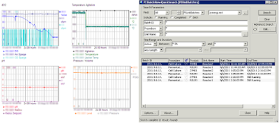
The Run Chart is basically what a chart-recorder spits out. In this day and age, it's what we call OSIsoft PI. You plot a parameter against time (called a trend), and when you do this, you get to see what's happening in sequential order. When you plot a lot of parameters on top of one another, you begin to understand sequence. Things that happen later cannot cause events that happened earlier. Say your online dissolved oxygen readings spiked below 5% for 10 seconds, yet your pO2 remains steady and the following viability measurement shows no drop off in cell viability, you can basically say that the dO2 spike was measurement error.

Here's an example of the modern-day run chart, it's called, "PI":


Run charts (i.e. PI) are crucial for solving immediate problems. A drifting pH probe can dump excess CO2 into a media-batched fermentor. Being able to see real-time data from your instruments and have the experience to figure out what is going on is key to troubleshooting large-scale cell culture and fixing the problem real-time so that the defect is not sent downstream.

Get #1 Biotech/Pharma PI Systems Integrator

As you can see, SPC concepts are timelessly applied today to cell culture and fermentation... albeit with new technology.

SPC - Process Flow Diagram/Pareto Charts

by Oliver Yu

So that little SPC Book goes into 7-tools to use, the next page goes into Process Flow Diagrams and Pareto charts.

Process Flow Diagram

The first tool appears to be the Process Flow Diagram[tm], where one is supposed to draw out the inputs and outputs of each process step. I suppose in the "Lean" world, this is the equivalent of value-stream mapping.

The text of the booklet calls it a

Pictoral display of the movement through a process. It simply shows the various process stages in sequential order.

Normally, I see this on a Powerpoint slide somewhere. And frankly, I've rarely seen it used in practice. More often, if we show this to consultants to get them up to speed.

Pareto Chart

The pareto chart is essentially a pie chart in bar-format. The key difference is that pie charts are for the USA Today readership while pareto charts are for real engineers -- this is to say that if you're putting pie charts in Powerpoint and you're an engineer, you're doing it wrong.

Pareto charts are super useful because they help figure out your most pressing issue. For example, say you're create a table of your fermentation failures:


So you have counted the number of observed failures alongside a weight of how devastating the failure is. Well, in JMP, you can simply create a pareto chart:


and out pops a pareto chart.


What this pareto chart shows you is the most important things to focus your efforts on. If you solve the top 2 items on this pareto chart, you will have solved 80% of your problems - on a weighted scale.

The pareto is a great tool for metering out extremely limited resources and has been proven extremely effective in commercial cell culture/fermentation applications.

SPC - Deming 14 Points for Management

by Oliver Yu

I was cleaning out my bookshelf and found this nifty little pocketbook.


Quality policies back then were not run-on paragraphs:

Dow Corning will provide products and services that meet the requirements of our customers. Each employee must be committed to the goal of doing it right the first time.

Page 4 contains Deming's 14 points for management; apparently, Deming didn't know that humans can remember in groupings of items in 3, 5, or 7:

1. Create constancy of purpose toward improvement of product and service.
2. Adopt the new philosophy. Acceptance of poor product and service is roadblock to productivity.
3. Cease dependence on mass inspection. Replace by improved processes.
4. End the practice of awarding business on basis of price tag alone.
5. Find problems and fix them. Continually reduce waste and improve quality.
6. Institute modern methods of on training on the job.
7. Institute modern methods of supervision.
8. Drive out fear.
9. Break down barriers between departments and locations.
10. Eliminate numerical goals, posters and slogans. Don't ask for new levels of productivity without providing new methods.
11. Eliminate work standards and numerical quotas.
12. Remove barriers that stand between the worker and his right to pride of worksmanship.
13. Institute a vigorous program of education and training.
14. Create a structure in top management that will push every day on the above 13 points.

Page 5 is an introduction to the seven tools described in the remaining 25 pages of this pocket book.